Machine Learning in Practice

This article was originally posted on LinkedIn on 8/23/2017

This post is the second in a series introducing machine learning. If you’re not familiar with the basics of machine learning and haven’t read my first post, start there.

In my last article, I gave a brief introduction to machine learning. But what does the process of machine learning actually look like? Here’s a simplified, step-by-step description of the process.

Data Wrangling

The first step of a machine learning task is “data wrangling,” also known as “data munging”. This is the process of taking input data, in whatever form it’s available, and translating it to a form that can be consumed by later steps in the process. This may include things like combining data from different places, sorting it, standardizing its form, correcting errors, and filling in missing values.

Feature engineering

Feature engineering is a very important part of machine learning. It’s the process of using domain knowledge to create features which can be used to make a machine learning algorithm work. A few of the types of questions that can go into creating useful features are:

• Of all the potential inputs I have from my system, which are likely to be relevant to the questions I’m trying to answer?
• Are there pieces of information I might attain from other sources that could be relevant?
• Can I apply some kind of processing to my input data to generate features that may be relevant? For example, if I have attributes x and y, might x / y be relevant? What about the change in x from the previous sample? Or the value of y relative to its average?

Data wrangling and feature engineering together make the process of data preparation. It’s a laborious, time-consuming process that requires patience and domain knowledge; a survey by CrowdFlower found that data scientists spend 60% of their time on “cleaning and organizing data.”

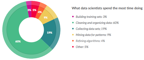
Incidentally, in the same survey, 57% of respondents said that data preparation was the least enjoyable part of data science; however, it is extremely important to the construction of a good model.

Feature selection

The next step is selection of a machine learning model and the features that will be used as inputs to the model. Feature and model selection are done in tandem; the full definition of a machine learned model is a combination of the model type used and the feature set on which it operates.

Feature selection is the process of winnowing down your collection of features to the set that gives the best model performance (while avoiding overfitting). There are a variety of feature selection algorithms which can be automatically applied, broadly falling into three classes. I’ll define them with some examples, but there are a vast number of different feature selection algorithms, and this will only scratch the surface.

Filter methods

Filter methods are the most conceptually simple type of feature selection method. In filter methods, some quantity is calculated to give a rough idea of how appropriate each potential feature is likely to be for prediction; for example, you might calculate the correlation between each feature and the variable to predict.

These methods serve to weed out variables that are less likely to have predictive power, and are much less computationally intensive than other methods. However, they will tend to select redundant variables. For example, if I have two variables x and y which are highly correlated with each other, they’re likely to have similar correlations to the target variable as well, but a model that already uses x for prediction will not be improved much by the addition of y, because they encapsulate the same information.

Wrapper methods

Wrapper methods evaluate subsets of variables, allowing the detection of interaction between variables. A very popular form of wrapper method for feature selection in regression models (such as linear or logistic regression) is stepwise regression. It’s a greedy algorithm that can be done in either the forward or backward direction.

In forward selection, you follow this basic procedure:

1. Start with a model with no features. For example, in linear regression, this would be a model consisting of just a single constant.
2. Fit a separate trial model for the addition of each potential feature (on the first pass, this will be N one-feature models, where N is the total number of features available). Choose the model which gives the most statistically significant improvement of the model.
3. Repeat step #2 above, adding a single feature each time, until no feature produces a statistically significant improvement.

Backward selection is just that process in reverse – start with a model including all features, and remove them one at a time until the model starts to get worse.

Because stepwise regression tests a very large number of different models, one must be very careful to avoid overfitting to the training data. It is important to carefully choose the appropriate criteria for “statistical significance”, such that addition or removal of a feature demonstrably affects the model accuracy more than random chance.

Embedded methods

Embedded methods are methods in which the machine learning model itself are biased in such a way that the best-fit model will contain the best subset of features. Regularization is the most typical type of embedded method.

In regularization, models are biased to smaller numbers of features using constraints. One example of regularization is LASSO, in which regression is performed under a constraint limiting the sum of the absolute values of the variable parameters.

Model selection

Model selection is choosing between different machine learning approaches that may be applicable to your problem. Model selection can be performed automatically, but is often an exploratory process for choosing the “best” model, where “best” can have different meanings. Here are a few examples of the many factors that might be considered in determining the model quality; the weights of the different factors in the final decision depend on the specifics of the problem.

• Interpretability: Is the model relatively concrete and low-dimensional, such that a human can understand how the features are combined to predict the output? More interpretable models can often lead to novel insights and aid decision making, for example, by suggesting business changes that the model suggests could make a desired outcome more likely.
• Accuracy: How well do predicted output match actual results in a test data set? See the next section for some discussion of model evaluation.
• Scalability: Can the model be applied to the volume of data required within the relevant time constraints? Certain types of models, while being more interpretable and accurate, may not lend themselves if the model needs to be applied to very large data sets and the results are needed in near real-time, for example.

Model selection also includes selecting model parameters. For example, for linear regression, our output is just a linear combination of our features. The full definition of the model includes all the parameters the input features are multiplied by; these can be automatically selected using the appropriate algorithm.

The range of possible model types and parameter fitting algorithms is very large; which models and algorithms are appropriate depends on the specific problem being solve.

Model evaluation

Model quality is evaluated on a separate set of data which was not involved in any part of the model training process. The criteria used to evaluate model quality depend on the type of model being trained, but for illustration, consider the loan default problem mentioned in part 1.

Assume the overally default rate is 5%, and we’ve built a model that classifies a borrower into one of “will default” or “will not default”. One simple metric for model quality is accuracy: “what percent of the time did my model predict correctly”? The problem with such a metric is easy to demonstrate: a model that simply classifies every borrower as “will not default” will have 95% accuracy!

In a binary classification problem like this one, precision and recall are important, complementary metrics.

• Precision is the fraction of positive predictions that are correct – that is, what percent of the borrowers who were predicted to default actually did?
• Recall is the fraction of true positives that are given positive predictions by the mdoel – that is, what percent of the borrowers who actually defaulted were predicted to do so by our model?

A highly predictive model will have both high prediction and recall; measures such as the F₁ score combine them into a single usable metric. Other metrics, such as AUC, are also used to get a comprehensive picture of model quality, balancing metrics like precision vs. recall.

Conclusion

This has been a brief overview of the steps involved in doing machine learning. It illustrates some of the major steps that will be common to machine learning tasks, but it’s not intended to be prescriptive; if anything, I hope I’ve sufficiently demonstrated that machine learning is not as simple as following a recipe.

While it’s possible that some day there will be a “black box” tool that reads in a bunch of data and spits out machine learned insights, modern machine learning methods require a great deal of knowledge and judgment on the part of the data scientist.